Today we’re tackling something that seems simple: how do you tell if a point is inside a triangle? I’ve got five things I want to do here:

Make it a story
This post will be long, with some detours and extra thoughts. But I think that’s the best way to get tricky stuff. A story keeps it interesting and helps you remember the important bits. So, this won’t just be words – it’ll be a journey with logic and aha moments.

Explain the basics simply

We’ll look at the building blocks and steps to figure out if a point’s in a triangle. Lots of people write about this, but I think they miss stuff or make it too quick. I’ll do it my way.

Focus on what you need

I’ll stick to the ideas that help solve this one question.

Show it’s not so simple

Even something small like this takes more understanding than you’d guess. I want to show that.

Try it out

This is from a book I’m writing. I’m testing if it works for readers.

Triangle

Just as the world is made up of atoms and molecules, at the heart of any 3D program lies the triangle. So, let’s begin our story with the triangle and explore why it’s so crucial for 3D graphics.

Let’s turn to the definition from Wikipedia:
A triangle is a figure consisting of three line segments, each of whose endpoints are connected. This forms a polygon with three sides and three angles.

Sounds terribly boring, doesn’t it? But don’t let that fool you – triangles are amazing. They’re behind your favorite 3D editor, video game, or big movie. Everything 3D on your screen? It’s all triangles doing the heavy lifting, turned into pixels in the end (they call that rasterization).

Here’s a heads-up: I might bend some geometry rules a bit. Serious math folks could get mad, but I think you can explain tricky stuff in a way that clicks faster than slogging through years of math classes.

So, let’s begin! We have the concept of a triangle: three points connected by three lines. Now, let’s break our molecule down into atoms.

Digression 1: Why the Triangle?

Time for a quick side trip (and there’ll be more, trust me) about why triangles are the go-to for 3D graphics, instead of something like a point or a circle.

Triangles can fake any shape
Even a circle! Pile up enough triangles, and you can make it look close enough to trick the eye.

Why not other shapes?

So, why not pick something else? Your screen’s just a bunch of pixels – tiny dots. Smooth shapes like circles don’t fit that world easily. You’ve got to fake them with something chunkier, like triangles.

Triangles are old friends

The properties of triangles have been well understood since the days of Pythagoras, making them a reliable and mathematically solid choice.

Easier to work with

Triangles make it easy to figure out things like light, shadows, and textures in graphics, way better than trickier shapes.

Tech loves them

All the modern graphics gear is built to handle triangles fast and smooth.

Side trip done – let’s get back to the atoms of our triangle, the points!

Point

A point marks a spot in space, plain and simple. It doesn’t have width, length, or thickness. But when we put it on paper, we make it a big dot anyway.

What can we do with points? In other words, what operations can we perform on points?

Can we add points?
You can technically add their parts x, y, z. But does it make sense? Not at all. So, adding points doesn’t really do much.

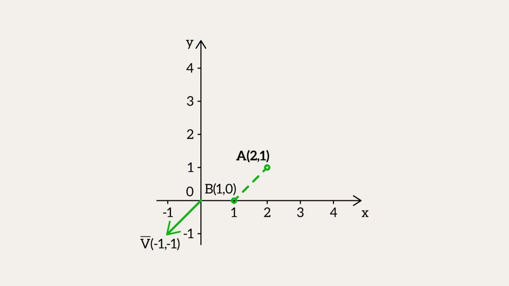
Can we subtract points?
Can we subtract points? Yes, and it gives us something new – a vector. You just take one point’s coordinates and subtract the other’s. Say you’ve got two points in 3D, and . Subtract them, and you get a vector .

Vector

Let’s take a quick look at vectors before we get back to points. A vector might seem like a point at first – same numbers – but it’s not. It’s about length and direction. Take two points, A and B. Subtract B – A, and you get a vector, , that shows the way from A to B. And if you measure that vector’s size – its magnitude, , you’ll get the distance between A and B.

If we draw the vector on a coordinate system, starting at and going to , we get a line that shows its direction.

Now, take point A and add vector to it. What do you get? Point B! So, it’s like the vector moves you from A to B.

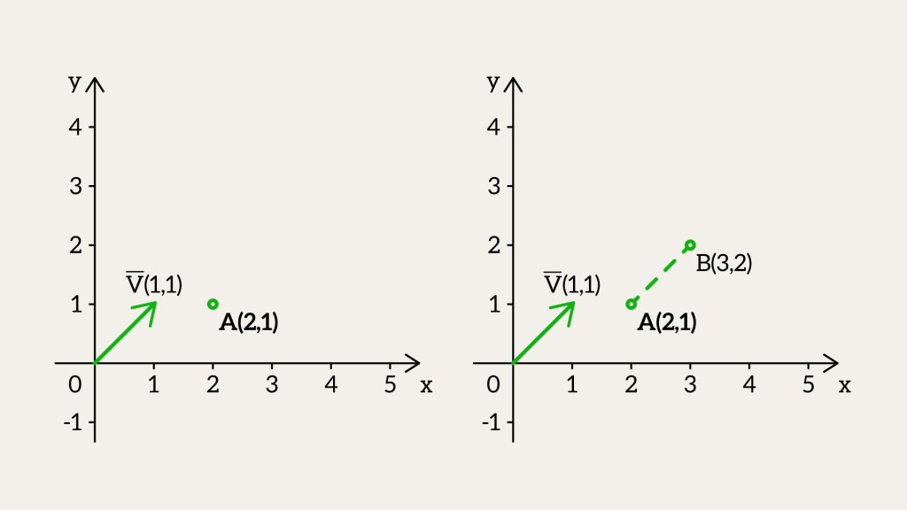
If we take point B and subtract vector from it, we end up back at point A. So, That’s how you can shift a point using a vector.

Now, if you flip the vector’s sign – make it negative – you get the same vector, just pointing the other way. For example, turns into .

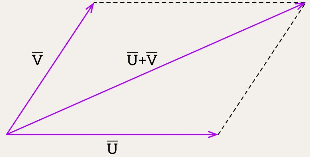
So, what’s possible with vectors? We can add them or subtract them. No big shock – the result is always another vector. But how do we picture it?

Take two vectors, and . To add them, imagine building a parallelogram. The diagonal of that shape shows their sum, .

Here’s how: start at the origin, then put at the end of . Draw lines parallel to and to finish the parallelogram. The diagonal from the origin? That’s .

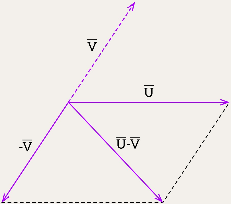
To show the difference between two vectors, think of it as adding one to the opposite of the other: . It’s still a parallelogram, just with flipped around.

Start with vector at the origin. Then take , reverse it to make , and put it at the end of . Draw the parallelogram using and as sides. The diagonal from the origin? That’s .

A Simple Trick to Remember Operations Between Points and Vectors

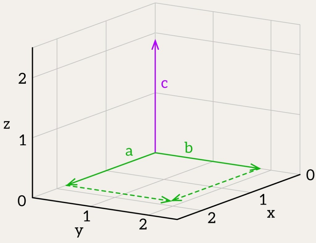
Want an easy way to handle points and vectors? Here’s a little trick: add a fourth number, w, to the usual x, y, z.

For a point, it’s (x, y, z, 1) – the w is 1.
For a vector, it’s (x, y, z, 0) – the w is 0.

With this, we can sort out all the operations between them. Let’s see how it works.

1. Subtracting two points
   Take two points, and . Subtract them: . That 0 at the end? It shows the result is a vector, not another point.
2. Adding two points
   What happens if we add two points, and ? You get . But that 2 at the end? It doesn’t mean anything here – no such thing as a “sum of points” exists in this world.
3. Subtracting a Vector from a Point
   Take a point and subtract a vector . You get . That 1 at the end? It means you’re still left with a point after moving by the vector.
4. Adding a Vector to a Point
   Take a point and add a vector . You get . That 1 at the end? It tells us the result is still a point after the shift.
5. Subtracting One Vector from Another
   Take two vectors, and . Subtract them: . That 0 at the end? It means you get a vector out of it.
6. Adding Two Vectors
   Take two vectors, and . Add them up: . That 0 at the end? It shows the result is still a vector.
7. Multiplying a Vector by a Scalar
   Take a vector and multiply it by a number . You get . That 0 at the end? It means it’s still a vector – just stretched or shrunk, keeping the same direction. (Unless is negative – then it flips the other way.)

That fourth coordinate, w, has another big role – we’ll get to it later. For now, let’s just keep it in mind as something neat. Going forward, we’ll drop it to keep things simple.

Digression 2: Point vs Vector classes

In programming, we usually split things into two classes: Point and Vector. But honestly, a lot of coders find that annoying. They’d rather treat a point like a radius vector – just another vector starting from the origin. That way, they can do all the math stuff, like adding or subtracting, without worrying about what’s a point and what’s a vector.

Say you’ve got two points, A and B, and you want the angle between them from the origin. You could write it like this:

Point O(0, 0, 0);
Vector vA = A-O;
Vector vB = B-O;
double angle = std::acos(dot(vA, vB) / (length(vA) * length(vB)));

But if you just treat A and B as radius vectors, it gets shorter:

double angle = std::acos(dot(A, B) / (length(A) * length(B)));

In the book, I separate vectors and points to keep the theory clear. But in the blog posts, I’ll use GLM, where both are just vec3, so I won’t bother making the distinction – it keeps things simpler.

Calculating Distance / Vector Length

Let’s tackle the distance between two points again. Take and . Picture a straight line between them. To measure it, think of the x-difference, , and the y-difference, . Square those, add them up – – and then take the square root. That’s your distance:

This works in 3D too. For points and , the distance is just: . Same idea, one more step.

Now, to find a vector’s length, pretend one point is the origin, . For a vector , its size is: .

Normals

Got a vector with a length ? Divide its components by . That gives you a unit vector, or a normal. We call this dividing step normalization. These normals have a length of 1 and point the way, making things simpler to figure out. Why are they big in computer graphics?

Lighting and Reflection
Normals show how light lands on surfaces – think brightness, shadows, or shiny reflections.

Shading
They help tricks like Phong shading make lighting look smooth and nice.

Reflection and Refraction
For stuff like water or glass, normals handle reflections and bending light.

Collisions and Physics
In games, they tell objects how to hit or bounce off each other.

Texturing
Normals fake extra detail in things like normal mapping, no extra shapes needed.

So, you’ve picked up the essentials – how to work with points and vectors, and even how to measure a vector’s length. Just a few more steps, and you’ll have this whole thing figured out!

Dot Product

What else can we do with vectors? There’s this thing called the dot product or scalar product – that’s super useful in geometry, physics, and graphics. Surprise: it gives you a number (or scalar), not a vector. It’s all about checking how much two vectors go the same way. Can we figure that out? Sure, here’s how:

It’s also called the projection product since it measures how much one vector follows another. Say we’ve got . Try it with any like , , , or – and you’ll get:

The answer’s always – could be , depending on . That’s how long stretches when you line it up with .

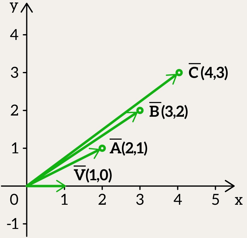
Put simply, the dot product here just looks at the horizontal part of – how much of it goes the same way as .

When one vector’s y-part is zero, like , it’s easy to see, like we showed before. But what if the y-part isn’t zero?

Let’s try two vectors: and . Let’s do something fun: rotate around so it sits on the x-axis. That zeroes out its y-part, leaving it pointing flat across. We’ll swing the same way too. Then, we just see how much lines up with this new .

We turn by , making it:
.

And gets the same twist, ending up as:
.

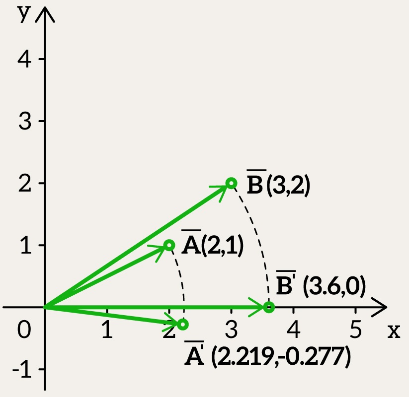
Now it’s simple: we just find the dot product between a vector flat on the x-axis and one with both x and y parts.

Since rotating doesn’t change the dot product, we calculate:

Put another way, is just , and shows how much stretches along when hits the x-axis. That’s .

So in the end, there is another way to calculate the dot product using the formula:

where:

• and are the lengths (magnitudes) of the vectors,
• is the angle between them,
• gives us the degree of alignment between the vectors.

The cosine function appears here because it naturally describes alignment:

• If two vectors point in the same direction, , so the dot product is maximal.
• If they are perpendicular, , meaning the dot product is zero (no alignment at all).
• If they point in opposite directions, , making the dot product negative.

Picture this: you’re in a dark room, holding a laser pointer. You aim it at a wall, but not straight on – it’s at an angle. The light doesn’t just hit one spot; it stretches across the wall. How long that streak is depends on your aim:

• When the laser is pointing directly at the wall, the projection is maximal, meaning the dot product is large. For unit vectors, the result is 1.
• When the laser is at an angle, the projection decreases, resulting in a smaller dot product.
• When the laser is perpendicular to the wall, there is no projection at all, and the dot product equals zero.
• When the laser is pointing in the opposite direction from the wall, the dot product is negative. For unit vectors, the result is -1.

Just a heads-up: we’re deep in dot product territory. It’s a big topic, full of details, but super important. If you get the dot product – really get it, with all its twists – it’ll make everything later so much easier. It’s the heart of all the cool stuff coming up.

What if we need to determine the angle between two vectors? We can solve for using the inverse cosine function:

Think of arccos as a way to convert a similarity measurement into an actual angle:

• If two vectors are identical, gives (perfect alignment).
• If they are perpendicular, gives .
• If they are opposite, gives .

This is extremely useful in applications like robotics, physics, 3D graphics, and AI, where finding angles between directions is crucial. The arccos function always returns an angle in the range from to (or from to radians).

Cross Product

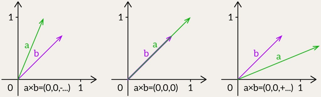
Now, let’s introduce the final operation you’ll frequently encounter: the vector product, also known as the cross product. Intuitively, this operation is simpler than the dot product because the result is something you can visualize – a new vector.

The result of the cross product is a vector , which is perpendicular to both vectors and .

For two vectors and , the cross product is defined as:

At this stage, I’d like to ask for your patience – don’t worry about where this formula comes from. Just memorize it for now, and later you’ll “teleport” back to it from another section.

The magnitude of the cross product represents the area of the parallelogram formed by vectors and :

The cross product can also be expressed as:

where is the unit normal vector perpendicular to the plane containing and .

The direction of (and ) is determined by the right-hand rule: curl the fingers of your right hand from to , and your thumb will point in the direction of .

is perpendicular to both and , and the cross product is not commutative: . Additionally, if and are parallel, then since .

Finally, let’s conclude our detour and return to our original task – determining whether a point is inside a triangle! At this stage, we have covered the basic geometric primitives: points, vectors, and operations on them. Now, with this knowledge, let’s finally solve our problem.

Is the point contained within the triangle? Cross Product Method

This method’s easy and makes sense, and it pulls together all the math we’ve gone over. For each edge of the triangle, we compute a cross product between the edge vector and the vector from the test point to one of the triangle’s vertices. That gives us three vectors that act like normals.

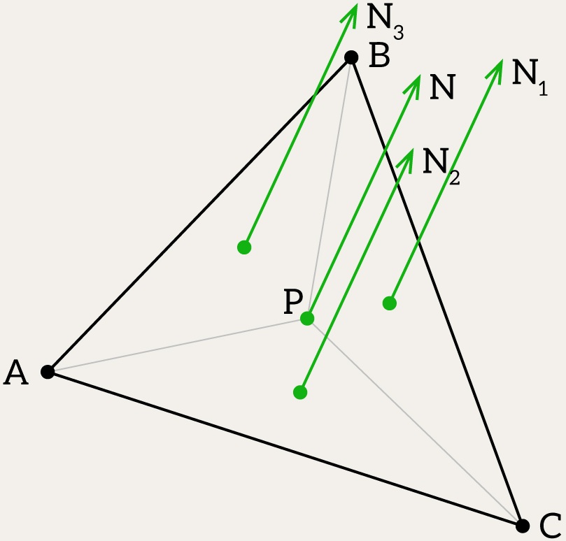
Each normal represents the orientation of the test point relative to a specific edge of the triangle.If is inside the triangle, all three cross-product normals should point in the same direction. If all three dot products have the same sign, then the point lies inside the triangle. Otherwise, at least one normal vector points in the opposite direction, indicating that is outside.

It is very important to note that this method works correctly only when the point lies in the plane of the triangle. This condition is often neglected in computer graphics since most algorithms do not require it. However, if you are working with engineering software and require precise calculations, it makes sense to add a check to ensure that the point lies in the triangle’s plane. In practice, such a check is usually performed earlier in the pipeline, before calling the point-in-triangle test, as part of collision detection, intersection tests, or geometric preprocessing.

bool isPointInsideTriangle(glm::dvec3 P, glm::dvec3 A, glm::dvec3 B, glm::dvec3 C, double epsilon) {
    // Compute the normal of triangle ABC and check if it's degenerate
    glm::dvec3 N = glm::cross(B - A, C - A);

    // Compute normals for sub-triangles PBC, PCA, PAB
    glm::dvec3 U = glm::cross(B - P, C - P);  // Normal of PBC
    glm::dvec3 V = glm::cross(C - P, A - P);  // Normal of PCA
    glm::dvec3 W = glm::cross(A - P, B - P);  // Normal of PAB

    // Compute scalar products of sub-triangle normals with the triangle normal
    double dot_u = glm::dot(U, N);
    double dot_v = glm::dot(V, N);
    double dot_w = glm::dot(W, N);

    return sameSigns(dot_u, dot_v, dot_w, epsilon);
}

The cross product method can run into trouble because of small math mistakes. These pop up when numbers get rounded off during multiplying and subtracting. It’s a problem when vectors are almost the same, especially in really thin (or as we call it – degenerate) triangles, and the answer might be off. Also, the final check – seeing if all normals point the same way – can mess up. If those normals shift and look almost at right angles because of these tiny errors, the test might call an inside point outside. epsilon helps by giving some extra space for those mistakes, making the checks better. You need to pick the right epsilon, though, or you might count outside points as inside or miss points that are barely inside.

Digression 3. Vector Operations: Functions vs. Operators

When handling vectors, libraries like GLM offer functions like dot and cross for scalar and vector products, instead of using signs like * or %. This has some good points. For one, dot and cross make it clear what math you’re doing, so the code’s easier to understand. Take dot(vA, vB) – it shows right away it’s a dot product. But vA * vB could mean different things, like multiplying by a number, doing it part by part, or even a dot product, depending on the setup. Same with cross(vA, vB) – it’s obvious it’s a cross product, while % isn’t something everyone knows and might remind people of division leftovers instead.

Another thing: functions like dot and cross make your code safer and easier to keep up. Signs like * can do lots of jobs – like multiplying by a number or working with matrices – which can mix things up if you’re not sure what’s meant or if the pieces don’t fit right. But dot and cross are built just for vectors, so you’re less likely to mess up. For instance, if you try dot with the wrong mix – like a vector and a plain number – a good library will catch it before the code even runs. With *, it might quietly do something you didn’t want.

Digression 4. Degenerate triangles

Degenerate triangles are bad – they don’t help anyone. They hold no real info. Either all their points sit on top of each other, or they line up straight. So, their area is pretty much zero. To spot these, we can figure out the triangle’s area using the cross product of its edge vectors and see if it’s tiny – below a small limit, area_epsilon. This way, we catch triangles that barely exist, whether because the points overlap or fall in a line, and kick them out before moving on. Here’s some code that checks if a triangle’s degenerate by looking at its area:

bool isTriangleDegenerate(glm::dvec3 A, glm::dvec3 B, glm::dvec3 C, double area_epsilon) {
    // Compute vectors along two edges of the triangle
    glm::dvec3 AB = B - A;
    glm::dvec3 AC = C - A;

    // Compute the cross product to get the normal vector
    glm::dvec3 N = glm::cross(AB, AC);

    // Compute the area as half the magnitude of the normal
    double area = 0.5 * glm::length(N);

    // Return true if the area is below the threshold, indicating degeneracy
    return area < area_epsilon;
}

So, we need to put this check at the beginning of our isPointInsideTriangle method. Next, we would like to address the problem mentioned at the beginning – we want to check if the point lies in the plane of the triangle.

Digression 5. Plane

A plane in 3D is like a big, flat sheet that goes on forever, set by a point and a normal vector. And guess what? The dot product – or projection product, as we call it now – saves the day again, tying all this geometry into a simple idea. Imagine a plane with a point and a normal vector , which stands straight up from the plane, at right angles to anything on it.

Now, take any point . We make a vector from to : . Since the normal is perpendicular to every vector on the plane, their dot product is zero: . Write that out, and you get . To tidy it up with a constant , it becomes , where .

struct Plane {
    glm::dvec3 N;  // A,B,C
    double D;
};

To check if a point lies on the plane, we evaluate:

• If the result equals 0 (within a small tolerance), the point lies exactly on the plane.
• If positive, the point is above the plane.
• If negative, the point is below the plane.

bool isPointOnPlane(glm::dvec3 P, Plane plane, double epsilon) {
    return std::abs(glm::dot(plane.N, P) + plane.D) <= epsilon;
}

To make a plane with a point and a normal vector, start with the plane equation. Plug in your point to figure out the constant .

Plane createPlane(glm::dvec3 P, glm::dvec3 N) {
    N = glm::normalize(N);
    double D = -glm::dot(N, P);
    return { N, D };
}

If you need to see if the point’s on the triangle’s plane, add this step after ruling out a bad triangle.

Think we’re done? Not even close. The method we went over is simple and pretty quick, but it’s got some weak spots, like we said before. Next, we’ll check out other ways to do this, and for that, we’ll need to dig even more into geometry basics.

Digression 6. Can you compute a cross product in 2D?

No, you cannot compute a cross product in a strictly two-dimensional space in the same way as in 3D – because the result is not a vector in 2D. However, if we extend the 2D vectors into 3D by assuming their -coordinates are zero and use the standard 3D cross product formula:

and set the -coordinates to zero, treating 2D vectors as lying in the -plane of 3D space, we obtain:

Since the only nonzero component is the -coordinate, we can define the 2D cross product as the scalar:

This scalar represents the signed area of the parallelogram formed by and .

• If a lies on the left from , the result is negative.
• If and are collinear, the result is zero.
• If a lies on the right from , the result is positive.

Thus, the signed area can be used to determine whether a 2D point is inside a 2D triangle. To do this, you need to compute the signed area of the triangle ABC and all the “sub-triangles” ABP, BCP, and CAP. If all the areas have the same sign, then the point lies inside the triangle.

bool isPointInsideTriangle(glm::dvec2 P, glm::dvec2 A, glm::dvec2 B, glm::dvec2 C, double area_epsilon) {
    // Compute the area of the triangle
    double triangleArea = area(A, B, C);

    // Check if the triangle is degenerate (area too small)
    if (std::abs(triangleArea) < area_epsilon)
        return false;

    // Compute areas of sub-triangles formed by point P
    double area1 = area(A, B, P);
    double area2 = area(B, C, P);
    double area3 = area(C, A, P);

    // Check if all sub-triangle areas have the same orientation (same sign)
    return sameSigns(triangleArea, area1, area2, area3, area_epsilon);
}

To get a triangle’s area using the 2D cross product, just take the absolute value of that cross product and cut it in half.

double area(glm::dvec2 A, glm::dvec2 B, glm::dvec2 C) {
    glm::dvec2 vec1 = B - A;
    glm::dvec2 vec2 = C - A;
    double crossProductValue = vec1.x * vec2.y - vec1.y * vec2.x;
    return 0.5 * crossProductValue;
}

Now, let’s finally return to where we started – the Triangle!

Triangle

Phew! We took a little detour, but now let’s return to the triangle. Consider a triangle defined by three vertices: , , and . Some useful properties we can compute are:

1. Lengths of sides, calculated using the distance formula:
   
   
   
2. Triangle normal, determining the orientation, given by the cross product:
   
3. Triangle area, calculated as half the magnitude of the normal vector:
   
4. Centroid, the geometric center, computed as the average of the vertices:
   Finding the centroid is simple, but how can we describe the position of any other point inside the triangle? For that, we use barycentric coordinates!

Barycentric Coordinates

Barycentric coordinates show where a point is in a triangle using weights. Think of a triangle with corners . Any point inside gets coordinates . Here are weights for each corner. A bigger weight means is closer to that corner. A smaller one means it’s farther. The weights always add up to 1: . If is right between and , it’s . So means doesn’t matter, and , mean it’s halfway between and .

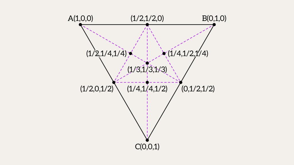
Picture a different triangle with the same barycentric coordinates for a point. They still tell us how it sits relative to the corners.

How do barycentric coordinates solve our first question? It’s pretty easy. If all the weights u, v, w are between 0 and 1, the point is inside the triangle.

Digression 7. Lines and Segments

Can we use barycentric coordinates for a line segment? For sure! It’s like with a triangle, just simpler. Picture a line with two ends, and . Any point on that line comes from mixing those two, using weights and . Here, is how much pulls, and is how much pulls. They always add up to 1: . If slides toward , gets bigger; if it heads toward , grows instead. This trick’s also called linear interpolation – or “lerp” for short (C++ has it now as std::lerp). For points and , it looks like this:

, where

For example: take . The weights come out as and . That means is pulling harder here.

Now try . You get and – perfect balance between and .

How do we figure out those weights and for a point between endpoints and ?

Start with the segment vector , and the vector from to , which is . Think of as sitting somewhere along the line:

Now, use the dot product with on both sides:

Solve for , and you get:

Then, the other weight is just .

Barycentric Coordinates: Triangle

Let’s figure out if point is inside triangle , but this time, let’s keep it really simple. Imagine you’re at , and you’ve got paths to and . Any point inside the triangle is like a mix of steps toward and .

We’ll use two vectors:
(the direction to )
(the direction to )

And one more:
(straight to )

The idea is, is some blend of and . Picture it like this: you walk a bit along , then a bit along , and land at . We write that as:

is your step along , and is your step along . If and are between 0 and 1, and they don’t add up to more than 1, is in the triangle.

So how do we find and ? Think of it as measuring how much leans toward each path. We can “ask” how much it matches and using dot products – like checking shadows:

• How much along ?
• How much along ?

This gives us two clues:

To find the coordinates, we solve the two equations above, and the results are:

Then, the last piece is:

If , , and are all between 0 and 1, is inside.

Keep in mind that this method, like the previous one, assumes that the point lies in the plane of the triangle.

bool isPointInTriangle(glm::dvec3 P, glm::dvec3 A, glm::dvec3 B, glm::dvec3 C, double epsilon) {
    // Define vectors along edges
    glm::dvec3 AB = B - A;
    glm::dvec3 AC = C - A;
    glm::dvec3 AP = P - A;

    // Compute the normal of triangle ABC
    glm::dvec3 N = glm::cross(AB, AC);

    // Compute dot products needed for barycentric coordinates
    double dotABAB = glm::dot(AB, AB);
    double dotABAC = glm::dot(AB, AC);
    double dotACAC = glm::dot(AC, AC);
    double dotAPAB = glm::dot(AP, AB);
    double dotAPAC = glm::dot(AP, AC);

    // Compute denominator
    double denom = dotABAB * dotACAC - dotABAC * dotABAC;
    if (std::abs(denom) < epsilon) 
        return false; // Denominator too small, unstable result
    
    double invDenom = 1.0 / denom;

    // Compute barycentric coordinates (v, w, u)
    double v = (dotACAC * dotAPAB - dotABAC * dotAPAC) * invDenom;
    double w = (dotABAB * dotAPAC - dotABAC * dotAPAB) * invDenom;
    double u = 1.0 - v - w;

    // Check if the point lies inside the triangle within epsilon tolerance
    return (u >= -epsilon) && (v >= -epsilon) && (w >= -epsilon);
}

This method finds barycentric coordinates using an inverse denominator, which is . Here, comes from the vector to times itself, is to times itself, and mixes them. If , it’s too tiny, so we stop and say – no dividing by almost zero! But when is really near an edge, those dot products can vary slightly, making , , or go a little under zero or over one, which might mess things up. So, we use a small in the check – , , – to give some room for those small mistakes and keep things right near the edges.

If you still think this is the end, it’s not! There is another method that is often used in more precise engineering applications.

Projection onto a 2D Plane

Every triangle in 3D lies flat on a plane, so we can shrink this problem down to 2D. Pick a plane – like the xy-plane, xz-plane, or yz-plane – and project everything onto it.

Here’s the trick: first, find the plane the triangle’s on. Check if the point’s near it, with a little room for error. If it is, we just need to see if it’s inside the triangle. Since the triangle’s flat in 3D, it’s a 2D question at heart. To keep it easy, we drop one coordinate from the triangle and the point, flattening them down.

Note that you need to add checks for triangle degeneracy and for whether the point lies on the plane of the triangle.

bool isPointInsideTriangle(glm::dvec3 P, glm::dvec3 A, glm::dvec3 B, glm::dvec3 C,
                           double epsilon, double area_epsilon)
{
    // Compute triangle normal and corresponding plane
    glm::dvec3 N = glm::cross(B - A, C - A);
    Plane plane = createPlane(A, N);

    // Select dominant axis for stable 2D projection
    glm::dvec3 absN = glm::abs(N);
    uint8_t dominantAxis = (absN.x > absN.y && absN.x > absN.z) ? 0 :
                           (absN.y > absN.z ? 1 : 2);

    auto project2D = [dominantAxis](glm::dvec3 v) -> glm::dvec2 {
        switch (dominantAxis) {
            case 0: return {v.y, v.z}; 
            case 1: return {v.x, v.z}; 
            default: return {v.x, v.y}; 
        }
    };

    // Project point onto plane and perform 2D point-in-triangle test
    glm::dvec3 projectedP = projectPointOntoPlane(P, plane);

    return isPointInsideTriangle(project2D(projectedP),
                                 project2D(A), project2D(B), project2D(C),
                                 epsilon);
}

We drop the coordinate with the largest component in the normal, since it contributes the least to variations across the triangle. The normal shows how the triangle is tilted in space, and its largest part points to the axis the plane is nearly perpendicular to. Removing that axis gives us a reliable 2D projection for checking point inclusion. Check “An Efficient Ray-Polygon Intersection” chapter in Graphics Gems 1.

The final thing is to project our point onto the plane, which follows the rule . We do this by sliding along the plane’s normal until it hits the plane at . That’s written as:
, where is how far we need to move.

Since is on the plane, it fits the equation:

Plug in , and you get:

Solve for :

Now, with , we find

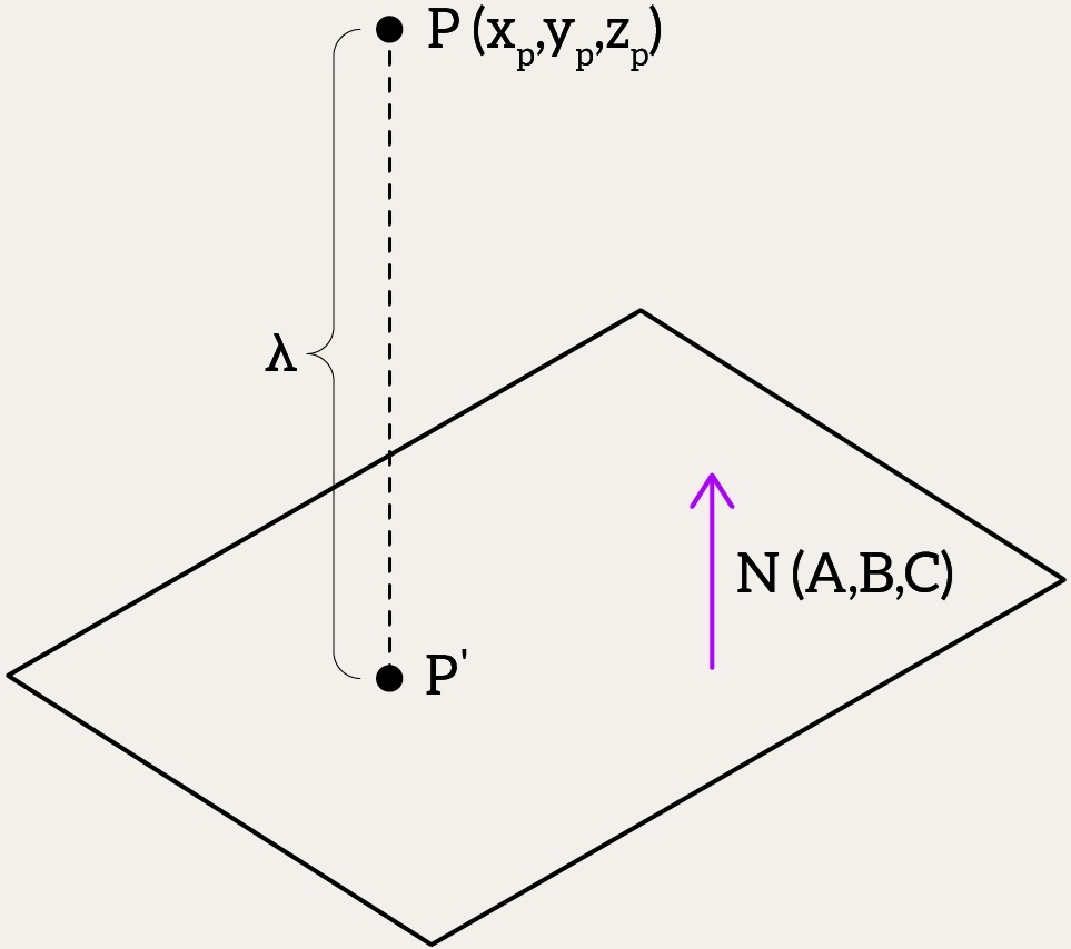
Thus, is the projection of onto the plane.

glm::dvec3 projectPointOntoPlane(glm::dvec3 P, Plane plane) {
    double lambda = (glm::dot(plane.N, P) + plane.D) / glm::dot(plane.N, plane.N);
    return P - lambda * plane.N;
}

Conclusion

Usually, this is where you’d expect a conclusion for the article – something about which method is better, which one’s worse, and why we picked this over that other one. But since this is just a snippet from a book, there’s no big wrap-up here. Instead, it rolls right into a more advanced, high-level problem down the road. So, for this post, the conclusion isn’t about crowning a winner among the methods. It’s more about how cool it is to break a problem down into tiny bricks and figure it out step by step with some neat math tools. What I really wanted to show here is how you can tackle the same task – checking if a point’s inside a triangle – in totally different ways. We’ve got the normals method, the barycentric coordinates trick, and that 2D projection move, each with its own strengths and trade-offs. They all get the job done, but they’re like different paths up the same hill. And by now, you’ve probably felt how much you need to know to code this stuff – vectors, dot products, floating-point nuances, and a touch of tolerance with epsilon to keep it all steady. It’s a lot of concepts to juggle! In the end, I hope messing around with this brought you some fun and maybe a little buzz from seeing how math and code can dance together.